Multi Cycle Kinetics

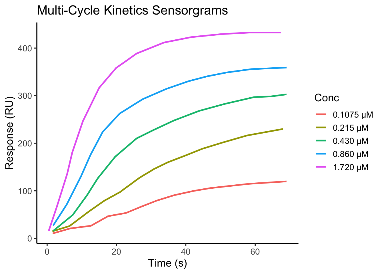
Now, let’s work through the data analysis of the other type of binding kinetics experiment we perform in Dr. Malkiat Johal’s lab. This type of experiment is a multi cycle kinetics experiment (MCK), and it is the most commonly used experiment in our lab. This type of experiment requires the immobilization of one chemical species (ligand) onto a sensor, recording the binding of the binding partner (analyte), and running an analyte concentration gradient with full regeneration of the underlying ligand surface between injections. The data we are working with today comes from my first first-author paper (Moonet et al., Anal. Chem. 2026). In this experiment, I was recording the binding between two polyelectrolytes (PEI and PAZO). PEI was used as the analyte in solution and PAZO the immobilized ligand. 5 concentrations of PEI were recorded, ranging from 1.72 uM to 0.1075 uM. Let’s import and visualize the raw data.

library(tidyverse)
library(minpack.lm)

PEI_1720 <- read.csv("PEI_1720.csv")
PEI_0860 <- read.csv("PEI_0860.csv")
PEI_0430 <- read.csv("PEI_0430.csv")
PEI_0215 <- read.csv("PEI_0215.csv")
PEI_01075 <- read.csv("PEI_01075.csv")

bind_rows(
  mutate(PEI_1720, Conc = "1.720 μM"),
  mutate(PEI_0860, Conc = "0.860 μM"),
  mutate(PEI_0430, Conc = "0.430 μM"),
  mutate(PEI_0215, Conc = "0.215 μM"),
  mutate(PEI_01075, Conc = "0.1075 μM")
) |>

ggplot(aes(Time, RU, color = Conc)) +
  geom_line(linewidth = 1) +
  labs(
    title = "Multi-Cycle Kinetics Sensorgrams",
    x = "Time (s)",
    y = "Response (RU)"
  ) +
  theme_classic(base_size = 14)

Gorgeous! We see clear, concentration-dependent binding.

The Mathematical Model

For a simple reversible interaction, we have

\[ A + B \rightleftharpoons AB \]

where

• (A) = PEI in solution (analyte)
• (B) = immobilized PAZO
• (AB) = surface-bound complex

The kinetics of a simple 1:1 Langmuir interaction are described by the differential equation

\[ \frac{dR}{dt} = k_{\mathrm{on}}\,C\left(R_{\max}-R\right) - k_{\mathrm{off}}R \]

where

• (R) is the SPR response (RU) at time (t),
• (R_{}) is the maximum binding response,
• (k_{}) is the association rate constant ((^{-1},)),
• (k_{}) is the dissociation rate constant ((^{-1})), and
• (C) is the analyte concentration.

During each association phase, the analyte concentration is constant,

\[ C(t)=C_0, \]

so the governing equation becomes

\[ \frac{dR}{dt} = k_{\mathrm{on}}\,C_0\left(R_{\max}-R\right) - k_{\mathrm{off}}R. \]

The analytical solution to this differential equation is

\[ R(t) = R_{\mathrm{eq}} \left( 1-e^{-k_{\mathrm{obs}}t} \right), \]

where

\[ k_{\mathrm{obs}} = k_{\mathrm{on}}C_0 + k_{\mathrm{off}} \]

and (R_{}) is the equilibrium response at that concentration.

Unlike single-cycle kinetics, each concentration is analyzed independently. Therefore, every sensorgram can be fit separately to determine the observed association rate constant ((k_{})) and the equilibrium response ((R_{})).

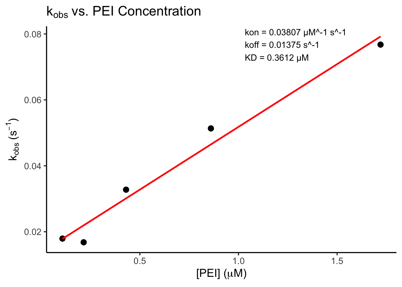
The relationship between (k_{}) and analyte concentration is linear,

\[ k_{\mathrm{obs}} = k_{\mathrm{on}}[PEI] + k_{\mathrm{off}}, \]

allowing the kinetic parameters to be determined by linear regression. The slope of the line gives the association rate constant ((k_{})), while the y-intercept gives the dissociation rate constant ((k_{})). The equilibrium dissociation constant is then calculated as

\[ K_D = \frac{k_{\mathrm{off}}}{k_{\mathrm{on}}}. \]

Now, let’s fit each association curve and extract the kinetic parameters!

library(tidyverse)
library(minpack.lm)

############################################################
# Concentrations (µM)
############################################################

datasets <- list(
  "1.7200" = PEI_1720,
  "0.8600" = PEI_0860,
  "0.4300" = PEI_0430,
  "0.2150" = PEI_0215,
  "0.1075" = PEI_01075
)

############################################################
# One-step association model
############################################################

assoc_model <- function(time, RUeq, kobs){
  RUeq * (1 - exp(-kobs * time))
}

############################################################
# Fit each concentration
############################################################

kineticfits <- map_df(names(datasets), function(conc){

  dat <- datasets[[conc]]

  fit <- nlsLM(
    RU ~ assoc_model(Time, RUeq, kobs),
    data = dat,
    start = list(
      RUeq = max(dat$RU),
      kobs = 0.03
    )
  )

  tibble(
    concentration = as.numeric(conc),
    RUeq = coef(fit)["RUeq"],
    kobs = coef(fit)["kobs"]
  )
})

############################################################
# Save fitted values
############################################################

write.csv(
  kineticfits,
  "kineticfits.csv",
  row.names = FALSE
)

print(kineticfits)

# A tibble: 5 × 3
  concentration  RUeq   kobs
          <dbl> <dbl>  <dbl>
1         1.72   442. 0.0768
2         0.86   376. 0.0513
3         0.43   346. 0.0328
4         0.215  348. 0.0168
5         0.108  178. 0.0179

############################################################
# Linear fit
############################################################

linearfit <- lm(kobs ~ concentration,
                data = kineticfits)

summary(linearfit)

Call:
lm(formula = kobs ~ concentration, data = kineticfits)

Residuals:
         1          2          3          4          5 
-2.454e-03  4.859e-03  2.644e-03 -5.131e-03  8.185e-05 

Coefficients:
              Estimate Std. Error t value Pr(>|t|)   
(Intercept)   0.013748   0.003101   4.433  0.02133 * 
concentration 0.038066   0.003493  10.897  0.00165 **
---
Signif. codes:  0 '***' 0.001 '**' 0.01 '*' 0.05 '.' 0.1 ' ' 1

Residual standard error: 0.004581 on 3 degrees of freedom
Multiple R-squared:  0.9754,    Adjusted R-squared:  0.9671 
F-statistic: 118.7 on 1 and 3 DF,  p-value: 0.001654

kon <- coef(linearfit)[2]
koff <- coef(linearfit)[1]
KD <- koff / kon

cat("\n")

cat("kon =", kon, "µM^-1 s^-1\n")

kon = 0.03806572 µM^-1 s^-1

cat("koff =", koff, "s^-1\n")

koff = 0.01374799 s^-1

cat("KD =", KD, "µM\n")

KD = 0.3611646 µM

############################################################
# Predicted line
############################################################

x <- seq(
  min(kineticfits$concentration),
  max(kineticfits$concentration),
  length.out = 200
)

pred <- tibble(
  concentration = x,
  kobs = predict(
    linearfit,
    newdata = data.frame(concentration = x)
  )
)


############################################################
# Plot
############################################################

ggplot(kineticfits,
       aes(concentration, kobs)) +

  geom_point(size = 3) +

  geom_line(
    data = pred,
    linewidth = 1,
    colour = "red"
  ) +

  labs(
    title = expression(k[obs]~"vs. PEI Concentration"),
    x = expression("[PEI] ("*mu*"M)"),
    y = expression(k[obs]~"(s"^{-1}*")")
  ) +

  annotate(
    "text",
    x = max(kineticfits$concentration)*0.60,
    y = max(kineticfits$kobs),
    hjust = 0,
    label = paste0(
      "kon = ", signif(kon,4), " µM^-1 s^-1\n",
      "koff = ", signif(koff,4), " s^-1\n",
      "KD = ", signif(KD,4), " µM"
    )
  ) +

  theme_classic(base_size = 14)

print(kineticfits)

# A tibble: 5 × 3
  concentration  RUeq   kobs
          <dbl> <dbl>  <dbl>
1         1.72   442. 0.0768
2         0.86   376. 0.0513
3         0.43   346. 0.0328
4         0.215  348. 0.0168
5         0.108  178. 0.0179

From the fitted values of k_{} and k_{}, we can take the ratio and get K_{}. Here, we get 0.3612 uM.

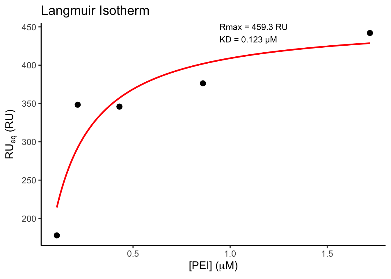
The Langmuir Model

Importantly, we also fit a value of RUeq for each concentration, the maximum response recorded from Importantly, this kinetic analysis does not for any effect of diffusion-contro and may oversimplify the kinetics and miss important mechanistic insight. The equilibrium response ((R_{})) obtained from each association fit can also be analyzed using a standard Langmuir adsorption isotherm. Each sensorgram can be fit to

\[ R(t)=R_{\mathrm{eq}}\left(1-e^{-k_{\mathrm{obs}}t}\right), \]

where (R_{}) is the fitted equilibrium response at each PEI concentration.

Because (R_{}) follows a Langmuir adsorption isotherm,

\[ R_{\mathrm{eq}} = R_{\max} \left( \frac{k_{\mathrm{on}}[\mathrm{PEI}]} {k_{\mathrm{on}}[\mathrm{PEI}]+k_{\mathrm{off}}} \right) = R_{\max} \left( \frac{[\mathrm{PEI}]} {[\mathrm{PEI}]+K_D} \right), \]

where

\[ K_D=\frac{k_{\mathrm{off}}}{k_{\mathrm{on}}}. \]

Thus, plotting (R_{}) versus PEI concentration and fitting the Langmuir isotherm provides an independent estimate of the equilibrium dissociation constant ((K_D)).

Let’s do the fit to this model!

###############################################################
# Fit
###############################################################

langmuir_fit <- nlsLM(
  RUeq ~ Rmax * concentration / (concentration + KD),
  data = kineticfits,
  start = list(
    Rmax = max(kineticfits$RUeq),
    KD = median(kineticfits$concentration)
  )
)

summary(langmuir_fit)

Formula: RUeq ~ Rmax * concentration/(concentration + KD)

Parameters:
      Estimate Std. Error t value Pr(>|t|)   
Rmax 459.31325   43.11192  10.654  0.00177 **
KD     0.12289    0.04862   2.528  0.08559 . 
---
Signif. codes:  0 '***' 0.001 '**' 0.01 '*' 0.05 '.' 0.1 ' ' 1

Residual standard error: 42.61 on 3 degrees of freedom

Number of iterations to convergence: 7 
Achieved convergence tolerance: 1.49e-08

###############################################################
# Extract fitted parameters
###############################################################

pars <- coef(langmuir_fit)

Rmax <- pars["Rmax"]
KD <- pars["KD"]

cat("Rmax =", Rmax, "RU\n")

Rmax = 459.3132 RU

cat("KD =", KD, "µM\n")

KD = 0.1228943 µM

###############################################################
# Generate fitted curve
###############################################################

fitcurve <- tibble(
  concentration = seq(
    min(kineticfits$concentration),
    max(kineticfits$concentration),
    length.out = 300
  )
)

fitcurve$RUeq <- predict(
  langmuir_fit,
  newdata = fitcurve
)

###############################################################
# Plot
###############################################################

ggplot(kineticfits,
       aes(concentration, RUeq)) +

  geom_point(size = 3) +

  geom_line(
    data = fitcurve,
    aes(concentration, RUeq),
    linewidth = 1,
    colour = "red"
  ) +

  labs(
    title = "Langmuir Isotherm",
    x = expression("[PEI] ("*mu*"M)"),
    y = expression(RU[eq]*" (RU)")
  ) +

  annotate(
    "text",
    x = max(kineticfits$concentration)*0.55,
    y = max(kineticfits$RUeq),
    hjust = 0,
    label = paste0(
      "Rmax = ", round(Rmax,1), " RU\n",
      "KD = ", signif(KD,3), " µM"
    )
  ) +

  theme_classic(base_size = 14)

As you can see, we get a different value for K_D depending on the model we choose to fit the data to. The value we get from the kinetic fit (let’s call it K_D,kin) and the Langmuir Isotherm (let’s call it K_D,eq) will differ specifically if there is a significant contribution of diffusion on the binding kinetics. When macromolecules take time to diffuse through solution, that time can actually be on the scale, or slower, than the binding reaction itself, becoming rate-limiting.

Quantifying diffusion

Using K_D values from both the kinetic and equilibrium models, we can quantify the effect of diffusion using the ratio, R, of the extracted kinetic models. Specifically, \[ R=\frac{K_{D,\mathrm{kin}}}{K_{D,\mathrm{eqm}}} \]. In the current experiment, we get R = 2.93, suggesting a substantial diffusion contribution to the reaction kinetics. The diffusion-control fraction (1-1/R) is 65.7%, indicating that the observed reaction is significantly diffusion-controlled, about 2/3 of the binding kinetics can be attributed to diffusion effects!