Permutation Test

Author

Ryan Mooney

The Task

Today, I will be running a permutation test using a data set from William Wolberg, Olvi Mangasarian. Nick Street, and W. Street in their paper “Nuclear feature extraction for breast tumor diagnosis” 1993 Published in Biomedical Image Processing and Biomedical Visualization.. The dataset was downloaded from UC Irvine Machine Learning Repository. The goal is to look at whether there is a correlation between diagnosis of a tumor and tumor size.

The Data

The data set compiled many features that were computed from a digitized image of a fine needle aspirate (FNA) of 529 breast masses. They recorded the following data:

ID number
Diagnosis (M = malignant, B = benign)

Ten real-valued features are computed for each cell nucleus:

a) radius (mean of distances from center to points on the perimeter)
b) texture (standard deviation of gray-scale values)
c) perimeter
d) area
e) smoothness (local variation in radius lengths)
f) compactness (perimeter^2 / area - 1.0)
g) concavity (severity of concave portions of the contour)
h) concave points (number of concave portions of the contour)
i) symmetry 
j) fractal dimension ("coastline approximation" - 1)

They provide standard errors and the “worst”, or the most extreme, value for each of the variables for each sample.

library(tidyverse)
library(readr)
library(praise)

tumor_data <- read_csv("data/wdbc.data")

colnames(tumor_data) <- c(
  "id", "diagnosis",
  "radius_mean", "texture_mean", "perimeter_mean", "area_mean", "smoothness_mean",
  "compactness_mean", "concavity_mean", "concave_points_mean", "symmetry_mean", "fractal_dimension_mean",
  
  "radius_se", "texture_se", "perimeter_se", "area_se", "smoothness_se",
  "compactness_se", "concavity_se", "concave_points_se", "symmetry_se", "fractal_dimension_se",
  
  "radius_worst", "texture_worst", "perimeter_worst", "area_worst", "smoothness_worst",
  "compactness_worst", "concavity_worst", "concave_points_worst", "symmetry_worst", "fractal_dimension_worst")

tumor_data

# A tibble: 568 × 32
         id diagnosis radius_mean texture_mean perimeter_mean area_mean
      <dbl> <chr>           <dbl>        <dbl>          <dbl>     <dbl>
 1   842517 M                20.6         17.8          133.      1326 
 2 84300903 M                19.7         21.2          130       1203 
 3 84348301 M                11.4         20.4           77.6      386.
 4 84358402 M                20.3         14.3          135.      1297 
 5   843786 M                12.4         15.7           82.6      477.
 6   844359 M                18.2         20.0          120.      1040 
 7 84458202 M                13.7         20.8           90.2      578.
 8   844981 M                13           21.8           87.5      520.
 9 84501001 M                12.5         24.0           84.0      476.
10   845636 M                16.0         23.2          103.       798.
# ℹ 558 more rows
# ℹ 26 more variables: smoothness_mean <dbl>, compactness_mean <dbl>,
#   concavity_mean <dbl>, concave_points_mean <dbl>, symmetry_mean <dbl>,
#   fractal_dimension_mean <dbl>, radius_se <dbl>, texture_se <dbl>,
#   perimeter_se <dbl>, area_se <dbl>, smoothness_se <dbl>,
#   compactness_se <dbl>, concavity_se <dbl>, concave_points_se <dbl>,
#   symmetry_se <dbl>, fractal_dimension_se <dbl>, radius_worst <dbl>, …

The Hypotheses

Today, I will be investigating the relationship between two variables: diagnosis (whether the tumor is malignant or benign) and mean tumor cell area. These variables are interesting because malignancy and benign tumors have different characteristics: malignant tumors are cancerous, they grow uncontrollably, invade nearby tissues, and can spread to other parts of the body, and benign tumors are non-cancerous, slow-growing, don’t invade surrounding tissue, and are typically treatable or harmless. Looking at cell area (and other variables) is interesting because it could give insight into which features can best be used to predict malignancy from small samples of tumor cells. The null hypothesis is that benign tumors and malignant tumors have cells of the same average area. The alternative hypothesis is that malignant tumors have larger average cell areas.

The statistic to test this difference will be difference in means between area in the benign and malignant tumor samples.

tumor_data |> 
  group_by(diagnosis) |> 
  summarize(ave_area = mean(area_mean))

# A tibble: 2 × 2
  diagnosis ave_area
  <chr>        <dbl>
1 B             463.
2 M             978.

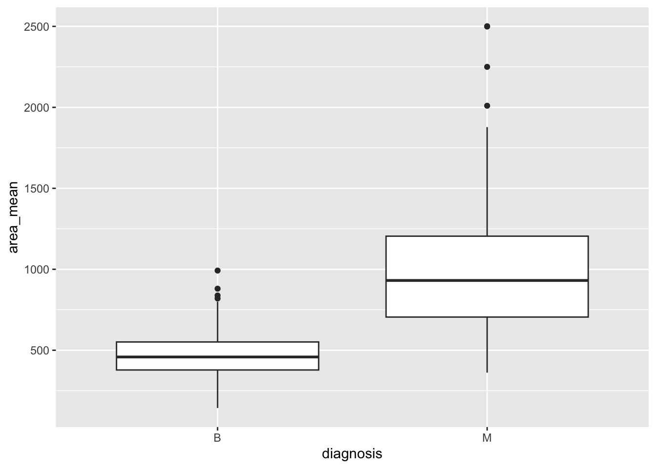
Here is a visual of the original relationship in the data.

tumor_data |> 
  ggplot(aes(x = diagnosis, y = area_mean)) + 
  geom_boxplot()

So, it looks like the mean area of malignant tumor cells is larger than that of benign tumor cells. However, is that generalizable to other breast tumors? Off to the permutation test!

The permutation test

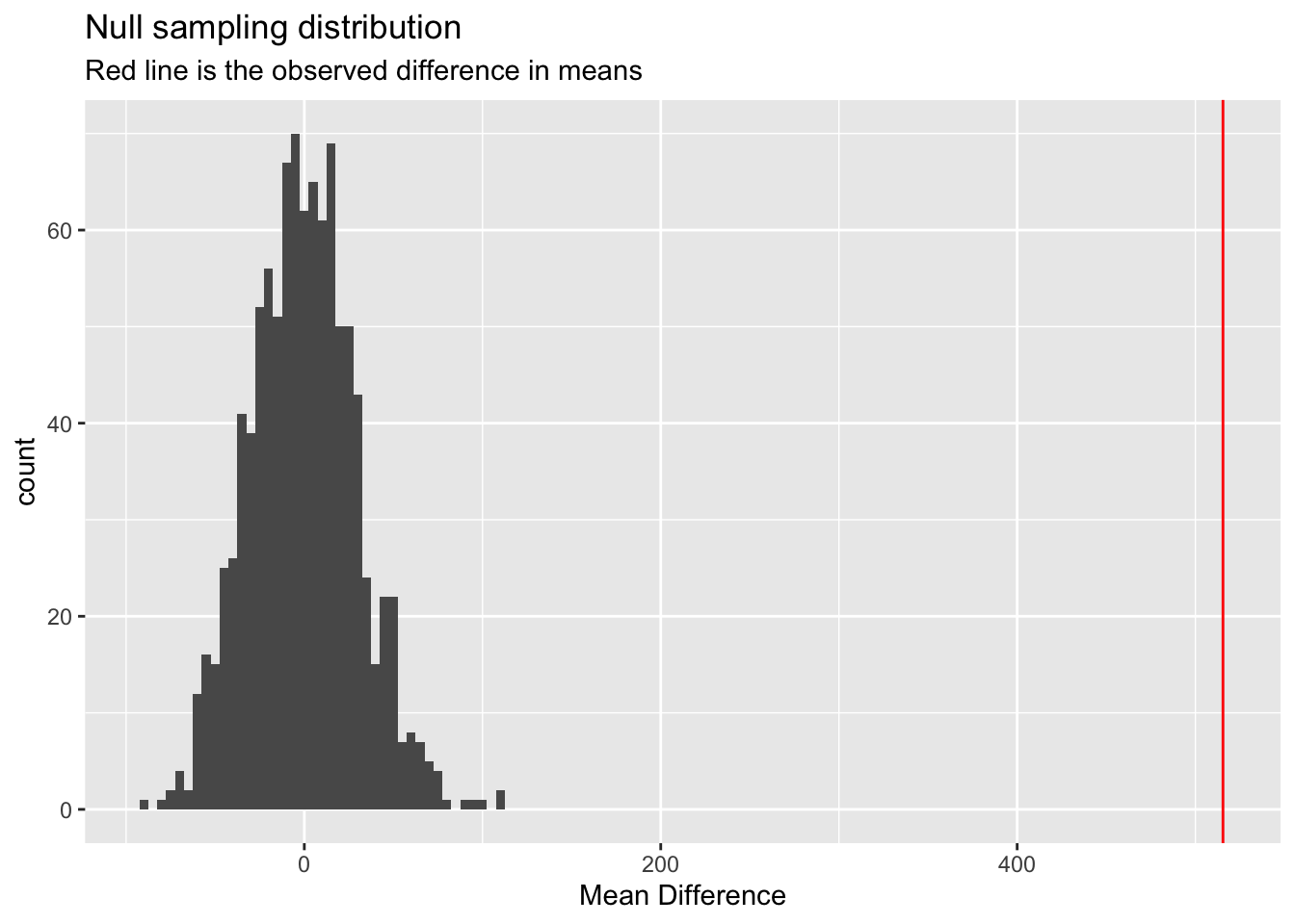
To start, I will generate a null sample distribution to compare the observed data with. This will serve as the basis of the generation of the p-value. The map(c(1:1000)) component performs the perm_data function 1000 times to generate a solid null distribution.

set.seed(47)
perm_data <- function(rep, data) {
  data |>
    select(diagnosis, area_mean) |>
    mutate(area_perm = sample(area_mean, replace = FALSE)) |>
    group_by(diagnosis) |>
    summarize(
      obs_mean  = mean(area_mean),
      perm_mean = mean(area_perm)) |>
    summarize(
      obs_mean_diff  = diff(obs_mean),
      perm_mean_diff = diff(perm_mean),
      rep = rep
    )
}

map(c(1:1000), perm_data, data = tumor_data) |> 
  list_rbind()

# A tibble: 1,000 × 3
   obs_mean_diff perm_mean_diff   rep
           <dbl>          <dbl> <int>
 1          515.         30.9       1
 2          515.        -52.8       2
 3          515.         63.0       3
 4          515.         24.5       4
 5          515.         -4.64      5
 6          515.          0.188     6
 7          515.         -6.70      7
 8          515.          9.85      8
 9          515.         45.6       9
10          515.        -55.7      10
# ℹ 990 more rows

Let’s look at the null sampling distribution and see where our experimental difference in means between malignant and benign tumor area lies.

set.seed(47)
perm_stats <- 
  map(c(1:1000), perm_data, data = tumor_data) |> 
  list_rbind() 

perm_stats |> 
  ggplot(aes(x = perm_mean_diff)) + 
  geom_histogram(binwidth = 5) + 
  geom_vline(aes(xintercept = obs_mean_diff), color = "red") + 
  labs(
    title = "Null sampling distribution",
    subtitle = "Red line is the observed difference in means",
    x = "Mean Difference"
  )

perm_stats |> 
    summarize(p_val = mean(perm_mean_diff > obs_mean_diff))

# A tibble: 1 × 1
  p_val
  <dbl>
1     0

The permutation test yielded a p-value of 0, indicating that the observed difference in mean cell size between malignant and benign breast tumors (515.479) did not occur once in 1,000 random permutations of the data. This extremely small p-value provides very strong evidence against the null hypothesis that benign and malignant tumors have the same average cell size. Thus, I claim that all malignant breast cancer cells have higher average sizes than benign cancer cells. This mean that average cell size could potentially serve as a potential quantitative metric for the rapid and automated classification of tumor malignancy.

That’s it!

Thanks for coming along for the ride today!

References

Street, W.N., Wolberg, W.H., & Mangasarian, O.L. “Nuclear feature extraction for breast tumor diagnosis.” (1993) Proc. SPIE 1905: Biomedical Image Processing and Biomedical Visualization. https://doi.org/10.1117/12.148698

Wolberg, W., Mangasarian, O., Street, N., & Street, W. “Breast Cancer Wisconsin (Diagnostic)” (1993) UCI Machine Learning Repository. https://doi.org/10.24432/C5DW2B