con_traffic <- DBI::dbConnect(
  RMariaDB::MariaDB(),
  dbname = "traffic",
  host = Sys.getenv("TRAFFIC_HOST"),
  user = Sys.getenv("TRAFFIC_USER"),
  password = Sys.getenv("TRAFFIC_PWD")
)SQL
The task
For today’s project, I will be working with data from the Stanford Open Policing Project pubished by Pierson, et al. (2020). I will be investigating a few of the many tables contained within the database.
First, let’s set up the connection to the traffic database and upload the needed packages for later analyses.
library(tidyverse)
library(DBI)
There are many tables in the database, including three that I am particularly interested in. These data tables are called “ca_statewide_2023_01_26”, “co_statewide_2020_04_01”, and “ny_statewide_2020_04_01”. These tables have all the statewide data for California, Colorado, and New York. Let’s compare!
To get a sense of the kinds of variables included in each set, let’s look at the start of the California table.
SELECT * FROM ca_statewide_2023_01_26 LIMIT 8;| raw_row_number | date | county_name | district | subject_race | subject_sex | department_name | type | violation | arrest_made | citation_issued | warning_issued | outcome | contraband_found | frisk_performed | search_conducted | search_person | search_basis | reason_for_stop | raw_race | raw_search_basis | raw_location_code |
|---|---|---|---|---|---|---|---|---|---|---|---|---|---|---|---|---|---|---|---|---|---|
| 1 | 2009-07-01 | Stanislaus | Modesto | other | male | California Highway Patrol | vehicular | Motorist / Public Service | NA | NA | NA | NA | NA | NA | 0 | 0 | NA | Motorist / Public Service | Other | Vehicle Inventory | 465 |
| 2 | 2009-07-01 | Stanislaus | Modesto | hispanic | female | California Highway Patrol | vehicular | Moving Violation (VC) | 0 | 0 | 0 | summons | NA | NA | 0 | 0 | NA | Moving Violation (VC) | Hispanic | Probable Cause (positive) | 465 |
| 3 | 2009-07-01 | Stanislaus | Modesto | hispanic | female | California Highway Patrol | vehicular | Moving Violation (VC) | 0 | 0 | 0 | summons | NA | NA | 1 | NA | other | Moving Violation (VC) | Hispanic | Probable Cause (positive) | 465 |
| 4 | 2009-07-01 | Stanislaus | Modesto | white | female | California Highway Patrol | vehicular | Moving Violation (VC) | 0 | 0 | 0 | summons | NA | NA | 0 | 0 | NA | Moving Violation (VC) | White | Probable Cause (positive) | 465 |
| 5 | 2009-07-01 | Stanislaus | Modesto | hispanic | male | California Highway Patrol | vehicular | Moving Violation (VC) | 0 | 0 | 0 | summons | NA | NA | 1 | NA | other | Moving Violation (VC) | Hispanic | Probable Cause (positive) | 465 |
| 6 | 2009-07-01 | Stanislaus | Modesto | hispanic | male | California Highway Patrol | vehicular | Moving Violation (VC) | 0 | 0 | 0 | summons | NA | NA | 0 | 0 | NA | Moving Violation (VC) | Hispanic | Probable Cause (positive) | 465 |
| 7 | 2009-07-01 | Stanislaus | Modesto | hispanic | female | California Highway Patrol | vehicular | Moving Violation (VC) | 0 | 0 | 0 | summons | NA | NA | 0 | 0 | NA | Moving Violation (VC) | Hispanic | Probable Cause (positive) | 465 |
| 8 | 2009-07-01 | Stanislaus | Modesto | other | female | California Highway Patrol | vehicular | Moving Violation (VC) | 0 | 0 | 0 | summons | NA | NA | 0 | 0 | NA | Moving Violation (VC) | Other | Probable Cause (positive) | 465 |
First, I’d like to make a plot to show how vehicular stops have changed over the years in California, Colorado, and New York.
I am going to UNION ALL three tables (co_statewide, ca_statewide, and ny_statewide), so that I can have one large data set with the needed data for the three states. This way, I can do the wrangling on the three states seperately and use the UNION ALL to combine those wrangled tables. I am focused on only vehicular stops, so I will include a WHERE type = ‘vehicular’ statement. I will also GROUP BY state and year(date) so that I will have seperate count information for each year in each state. I will store the following wrangled data in a dataframe called stops_per_year. Let’s do it!
SELECT
    'Colorado' AS state,
    YEAR(date) AS year,
    COUNT(*) AS total_stops
FROM co_statewide_2020_04_01
WHERE type = 'vehicular' AND YEAR(date) IS NOT NULL AND YEAR(date)>2008
GROUP BY state, YEAR(date)

UNION ALL

 SELECT
    'California' AS state,
    YEAR(date) AS year,
    COUNT(*) AS total_stops
FROM ca_statewide_2023_01_26
WHERE type = 'vehicular'
GROUP BY state, YEAR(date)

UNION ALL

SELECT
    'New York' AS state,
    YEAR(date) AS year,
    COUNT(*) AS total_stops
FROM ny_statewide_2020_04_01
WHERE type = 'vehicular'
GROUP BY state, YEAR(date)

ORDER BY year, state;
Now we can visualize the data! Let’s see how the states compare when it comes to total stops per year!
ggplot(stops_per_year,
       aes(x = year, y = total_stops, color = state)) +
  geom_line() +
  geom_point() +
  scale_x_continuous(breaks = 2009:2020) +
  labs(
    title = "Vehicular Stops in CA, CO, NY",
    x = "Year",
    y = "Stops",
    color = "State"

  )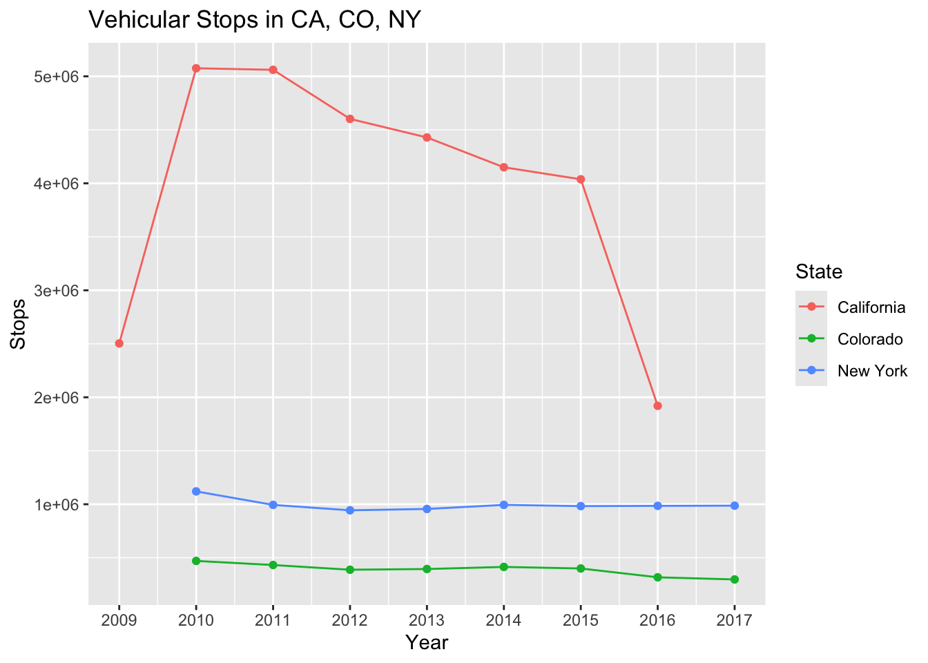
So, overall, California has more vehicular stops than Colorado and New York, and also has some more variation from year to year. Importantly, this is skewed upwards in the case of California because it has a much larger population! It is also likely true that for California, the years 2009 and 2016 have partial data, given their sudden drops from the rest of the data.
Next, now that I am more familiar with how these tables are organized and the specific variables available, I am interested in investigating California more closely to observe some more trends. I am interested how gender affects citation rates, as in how often do men get a citation when they are pulled over compared to women?
SELECT
    subject_sex,
    COUNT(*) AS n_stops,
    SUM(citation_issued) AS n_with_citation,
    COUNT(*) - SUM(citation_issued) AS n_without_citation,
    AVG(citation_issued) AS citation_rate
FROM ca_statewide_2023_01_26
WHERE subject_sex IN ('male', 'female')
GROUP BY subject_sex
ORDER BY subject_sex;
Let’s plot it!
ggplot(ca_sex_citations,
       aes(x = subject_sex, y = citation_rate)) +
  geom_col() +
  geom_text(
    aes(label = citation_rate),
    vjust = -0.5)+
  labs(
    title = "Citation Rate by Driver Sex in California",
    x = "Driver Sex",
    y = "Citation Rate"
  )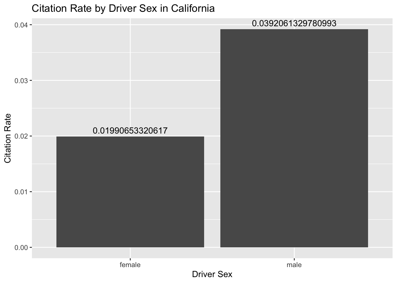
From the above analysis, it is seen that males get citations when they are stopped more often than females. There are likely many variables going into this rate difference. This could be due to men being more aggressive or impulsive drivers. I was interested and did some quick research on this, and it has been found that younger drivers, those with powerful cars, and those with “macho” personalities are more likely to drive agressively (Krahé & Fenske, 2001). This lines up to my calculation of California citation rates. Interesting!
Notably, these citation rates seem really low, so this is likely a variable that is not often included in the data set, but from the sample we have, the relative proportion of citations given to men and women are likely accurate.
From the analyses today, we can see that California has higher vehicular stops over time than Colorado and New York, and that males have higher citation rates than females in California. There are many, many variables that go into these kinds of analyses. These variables include population size, in the case of the first analysis, differences in driving behavior across states, and likely more social-related perception variables in the case of the difference in citation rates between men and women.
dbDisconnect(con_traffic, shutdown = TRUE)Thanks for coming along for the ride today!
References
Krahé, B., & Fenske, I. Predicting aggressive driving behavior: The role of macho personality, age, and power of car. Aggressive Behavior: Official Journal of the International Society for Research on Aggression, 28(1), 21-29. (2002).
Pierson, E., Simoiu, C., Overgoor, J. et al. A large-scale analysis of racial disparities in police stops across the United States. Nat Hum Behav 4, 736–745 (2020).